A robust method for copy number variation detection on dried blood spots.
Tutorial
# In R:
# Load iPsychCNV package
library(iPsychCNV)

 Run iPsychCNV Package
## Creates a mock data that simulates Infinium PsychArray BeadChip from Illumina.
## Mock data uses same SNP position as PsychArray chip.
MockCNVs <- MockData(N=1, Type="Blood", Cores=1)


# Running iPsychCNV on mock data.
CNVs <- iPsychCNV(PathRawData=".", Cores=1, Pattern="^MockSample*", Skip=0)

# PathRawData: Data path.
# Cores = 1, number of CPUs to be used.
# Pattern = "^MockSample*". Scan for the pattern in a given folder.

 EVALUATE PERFORMANCE
# Test and evaluate three methods using long mock data.
CNV.Prediction <- RunLongMock(Name="All", Method="All",
HMM="/media/NeoScreen/NeSc_home/share/Programs/penncnv/lib/hhall.hmm",
Path2PennCNV="/media/NeoScreen/NeSc_home/share/Programs/penncnv/")
iPsychCNV prediction. Gada prediction. PennCNV prediction PFB 0.5 for each SNP (PennCNV NO). PennCNV prediction PFB calculated for each SNP (PennCNV NA).
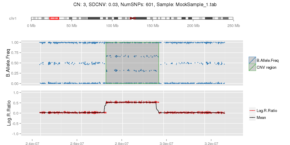
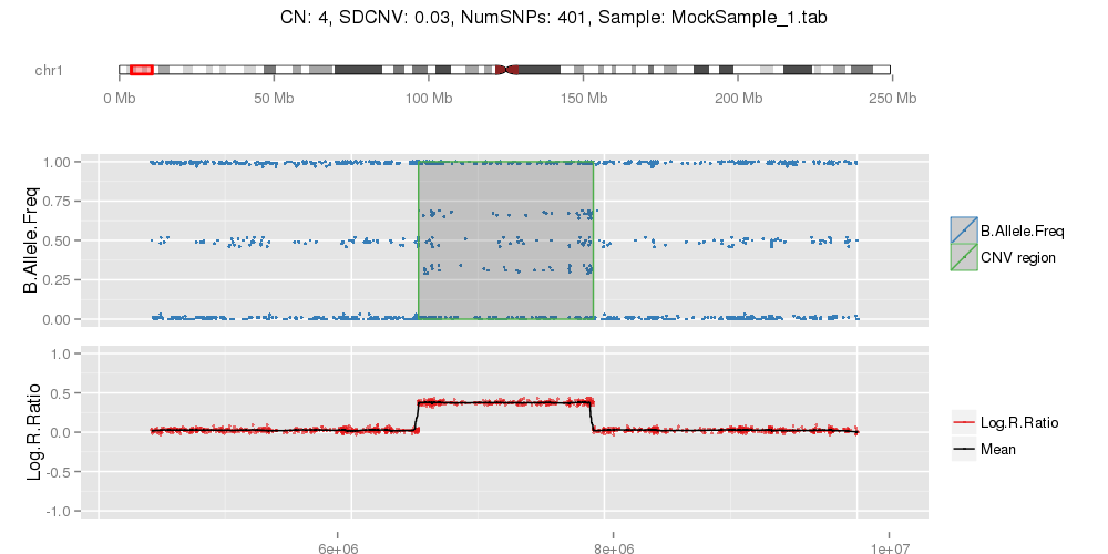
# Plotting individual CNVs from a data.frame
PlotCNVsFromDataFrame(DF=CNVs.Good[1:4,], PathRawData=".", Cores=1, Skip=0, Pattern="^MockSamples*")
Example of mock CNV with CN = 0. Example of mock CNV with CN = 1. Example of mock CNV with CN = 3. Example of mock CNV with CN = 4.
Long Mock
# Long mock has only one chromosome, and doesn't use PsychArray chip information.
# It is created to test combination of LRR and BAF found in DBS data.
# Input for long mock. More variables can be included.
# For example: Size=c(100, 300, 600, 2000)
CNVDistance=1000 # Distance among CNVs.
Type=c(0,1,2,3,4) # CNV copy number.
Mean=c(-0.6, -0.3, 0.3, 0.6) # CNV LRR mean.
Size=c(300, 600) # CNV number of SNPs.
Method = "iPsychCNV" # Method used
Name="LongMock" #
CNVMean=0.3 # If method has no CNV mean output.
Name <- paste(Name,"_",Method, "_LongMockResult.png", sep="", collapse="") # png plot name.
# Running long mock step by step
LongRoi <- MakeLongMockSample(CNVDistance, Type, Mean, Size)
# Reading long mock to an object in R.
Sample <- read.table("LongMockSample.tab", sep="\t", header=TRUE, stringsAsFactors=F)
# Running iPsychCNV on long mock data.
PredictedCNV <- iPsychCNV(PathRawData=".", Pattern="^LongMockSample.tab$", Skip=0)
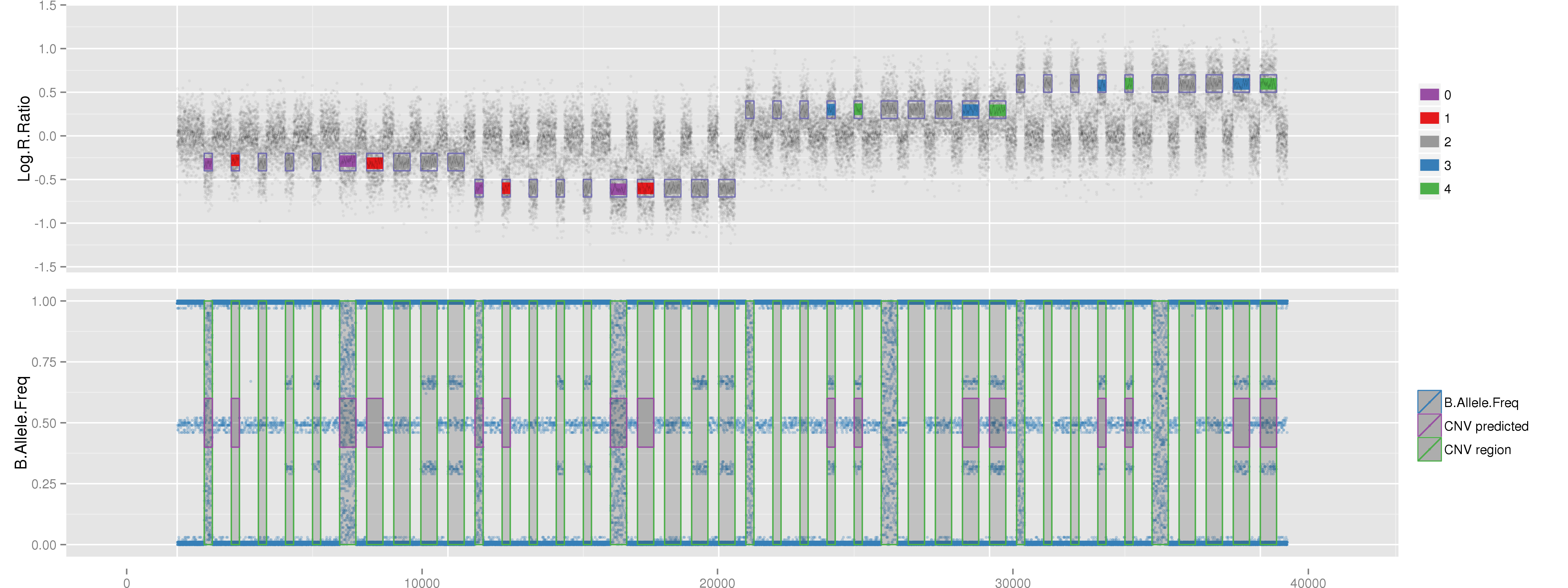
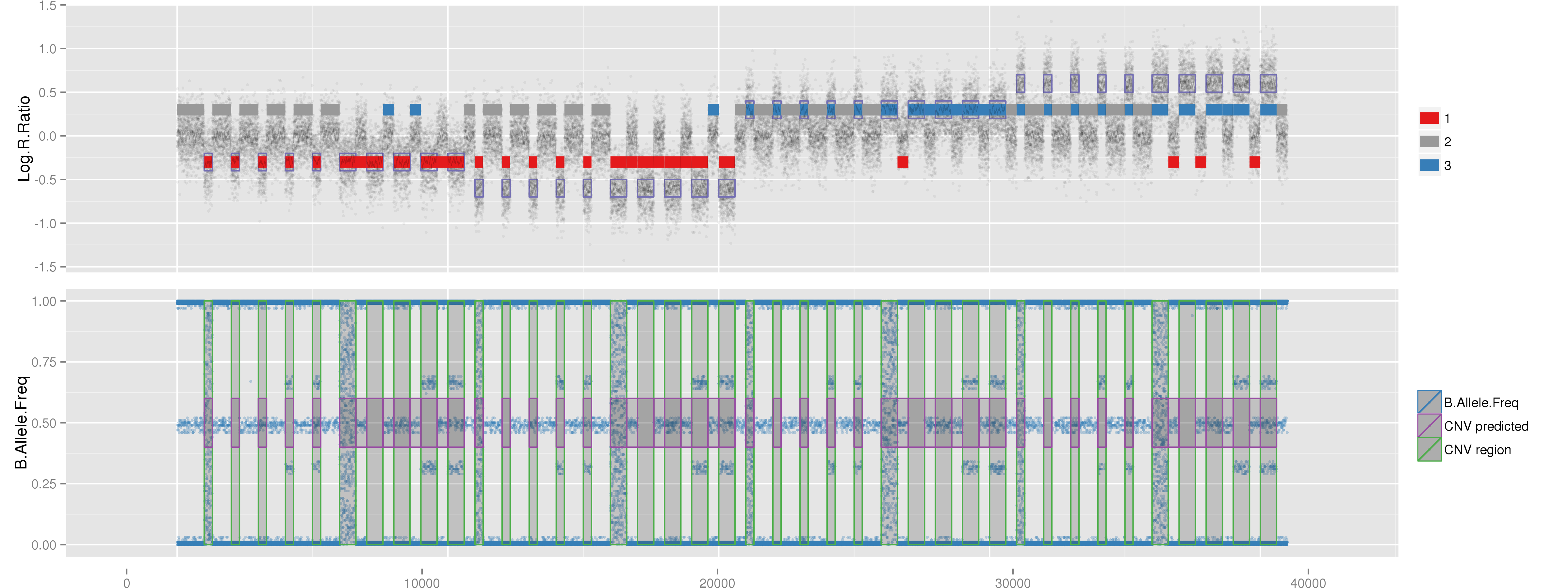
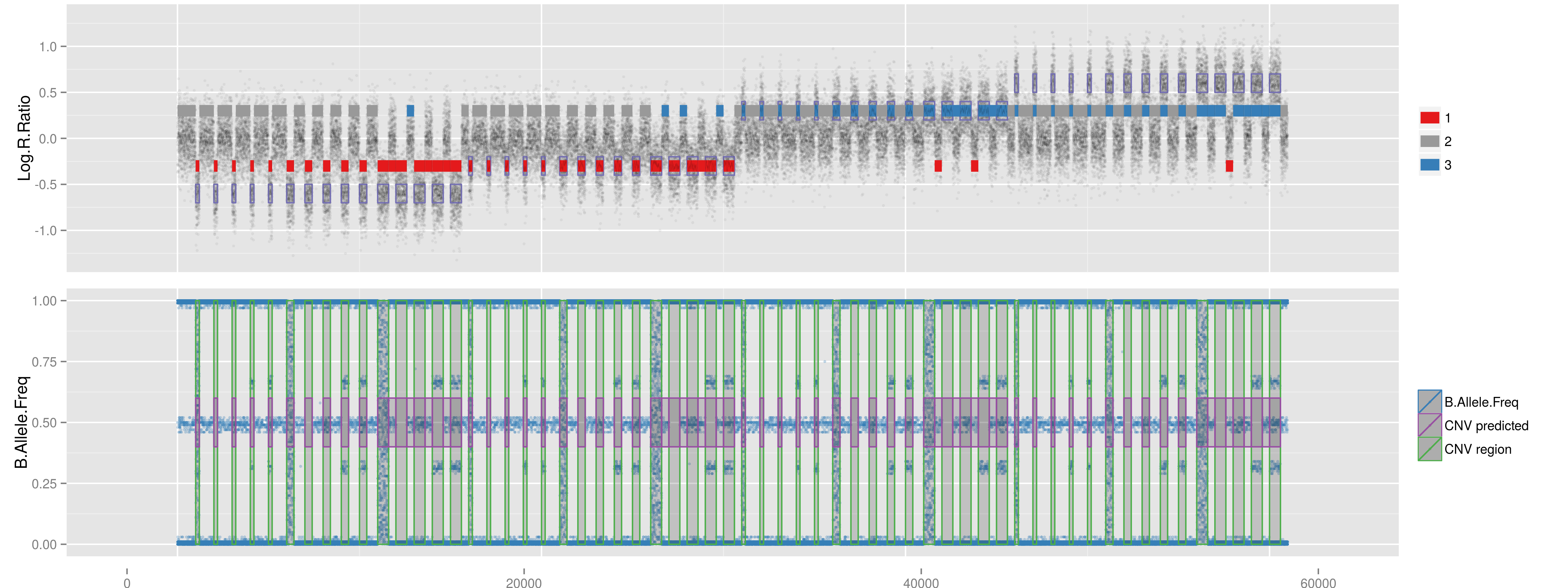
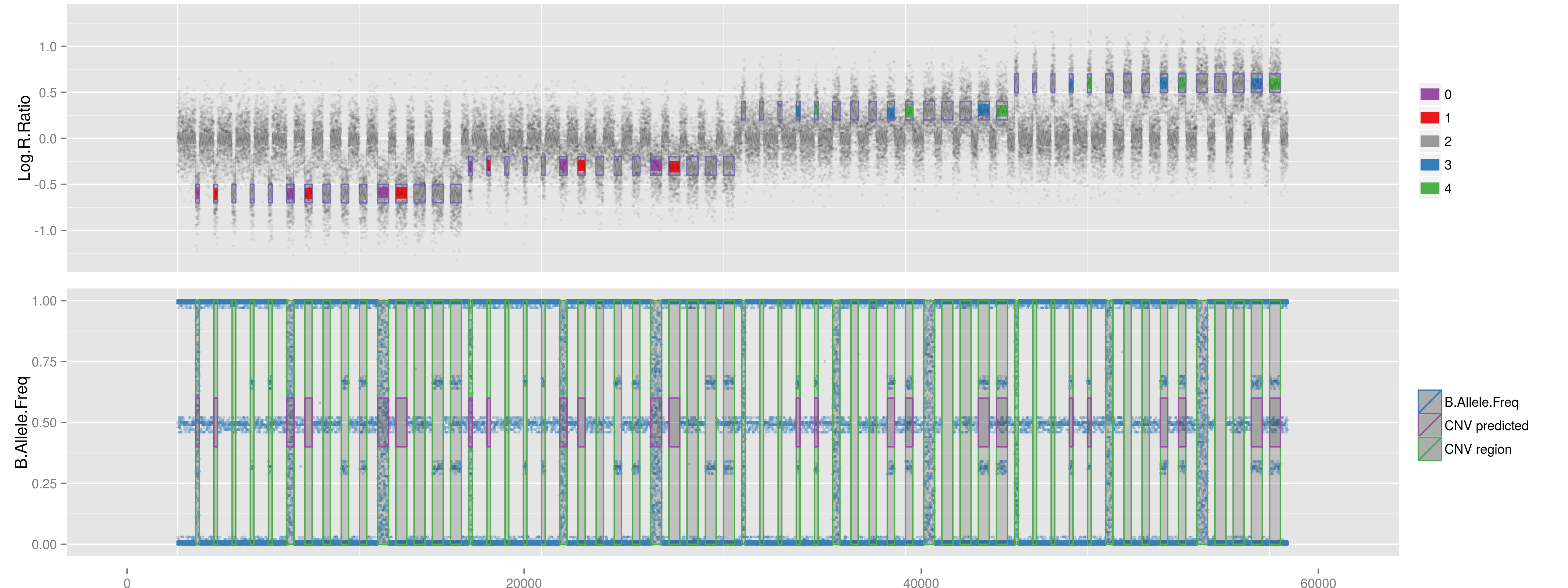
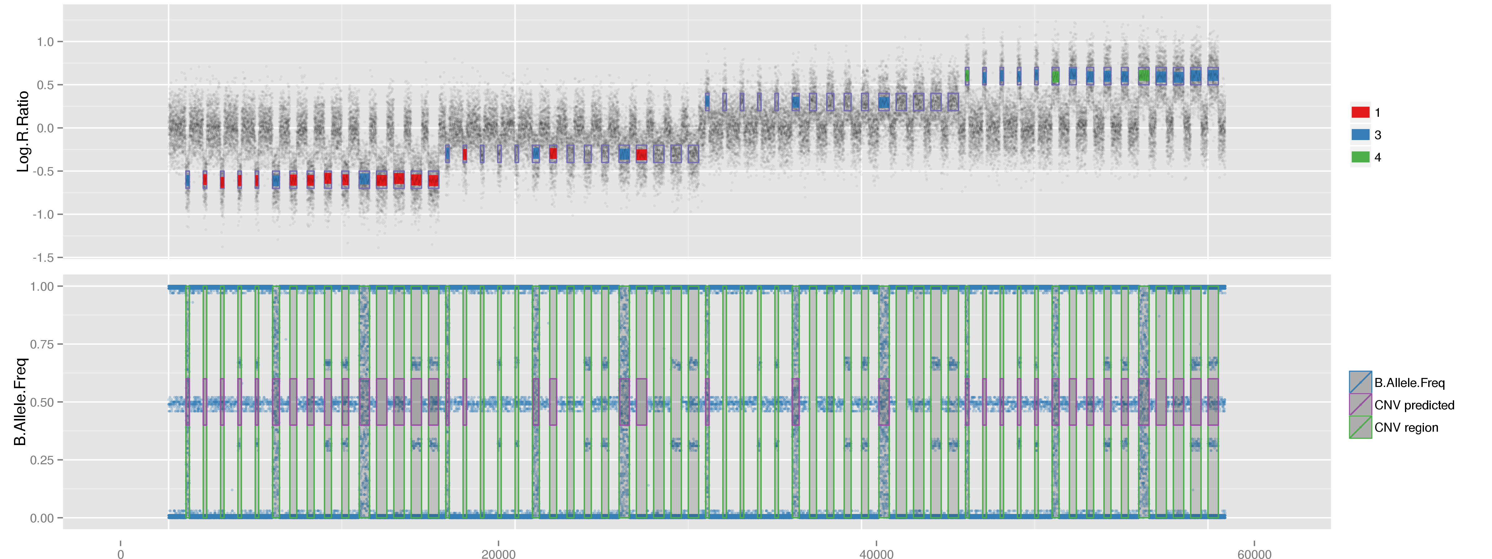
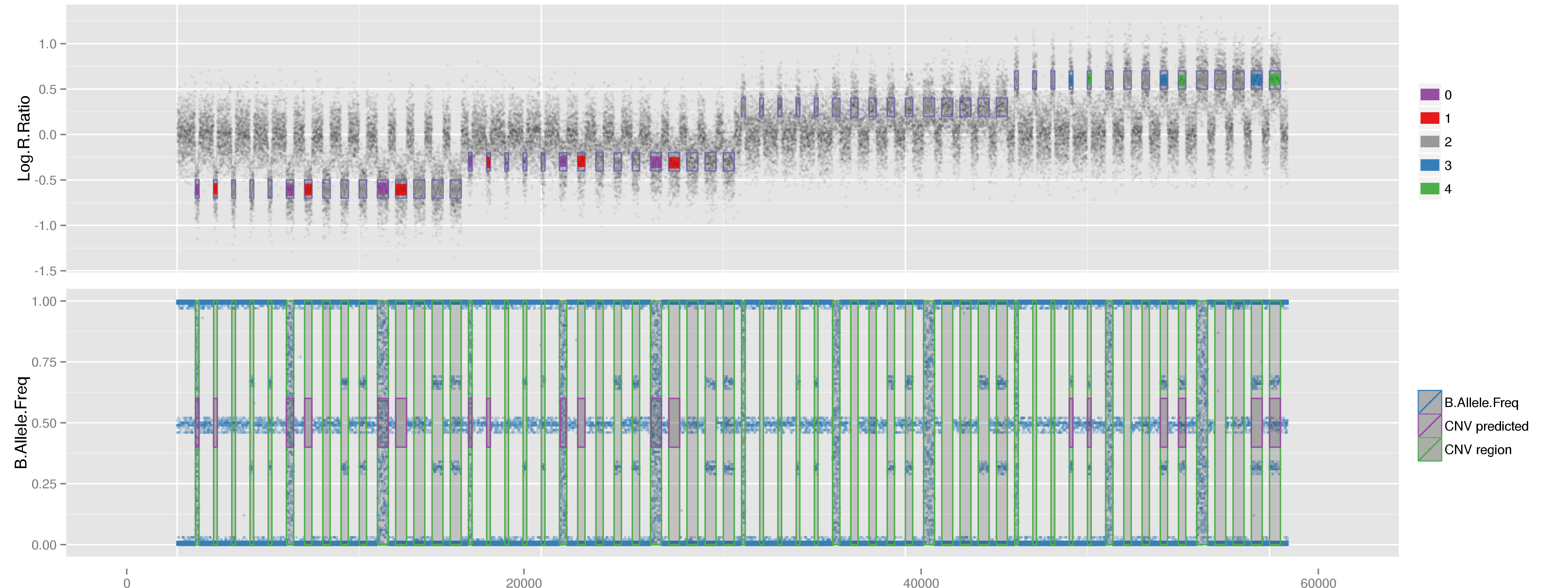
# Plotting LRR and BAF from
PlotLRRAndCNVs(PredictedCNV, Sample, CNVMean, Name=Name, Roi=LongRoi)
# Evaluating CNVs
CNVs.Eval <- EvaluateMockResults(LongRoi, PredictedCNV)
# Print ROC curve.
plot.roc(CNVs.Eval$CNV.Predicted, CNVs.Eval$CNV.Present, percent=TRUE, col="#1c61b6", print.auc=TRUE)
iPSYCHCNV STEP By STEP
# Function to read sample.
Mock.chr22 <- ReadSample(RawFile="MockSample_1.tab", skip=0, LCR=FALSE, chr=22)
# Function to find CNVs.
Mock.chr22.CNVs <- FindCNV.V4(ID="Test", MinNumSNPs=10, CNV=Mock.chr22)
# Function to validate CNVs.
Mock.chr22.CNVs.validation <- FilterCNVs.V4(CNVs=Mock.chr22.CNVs, MinNumSNPs=10, CNV=Mock.chr22, ID="Test")
Merge CNVs
# Using low penvalue to break CNV prediction.
Mock.chr22.CNVs <- FindCNV.V4(ID="Test", MinNumSNPs=10, CNV=Mock.chr22, CPTmethod="meanvar", penvalue=10)
# Second and Third CNV should be merged. Gap of only 11 SNPs or 47171 bp.
str(Mock.chr22.CNVs)
'data.frame': 5 obs. of 10 variables:
$ Start : int 24583365 32009612 33430734 38864287 45309851
$ Stop : int 25938025 33383563 35786182 39385595 46854398
$ CNVMean : num -0.454 0.387 0.391 0.428 0.379
$ StartIndx: num 1999 4006 4424 5999 7999
$ StopIndx : num 2400 4413 4800 6139 8600
$ Length : int 1354660 1373951 2355448 521308 1544547
$ NumSNPs : num 401 407 376 140 601
$ Chr : int 22 22 22 22 22
$ ID : chr "Test" "Test" "Test" "Test" ...
$ CN : num 1 3 3 3 3
Mock.chr22.CNVs.merged <- MergeCNVs(Mock.chr22.CNVs, MaxNumSNPs=50)
str(Mock.chr22.CNVs.merged)
'data.frame': 4 obs. of 10 variables:
$ Start : int 24583365 32009612 38864287 45309851
$ Stop : int 25938025 35786182 39385595 46854398
$ StartIndx: num 1999 4006 5999 7999
$ StopIndx : num 2400 4800 6139 8600
$ Length : int 1354660 3776570 521308 1544547
$ NumSNPs : num 401 794 140 601
$ CNVMean : num -0.454 0.387 0.428 0.379
$ Chr : int 22 22 22 22
$ ID : chr "Test" "Test" "Test" "Test"
$ CN : num 1 3 3 3
Filter CNVs from other methods
# It is possible to validate CNVs using prediction from other methods.
# For example, if you have PennCNV results it is possible to run the filter to collect CNV variables
#(that are required to run support vector machine) and get a preliminary evaluation.
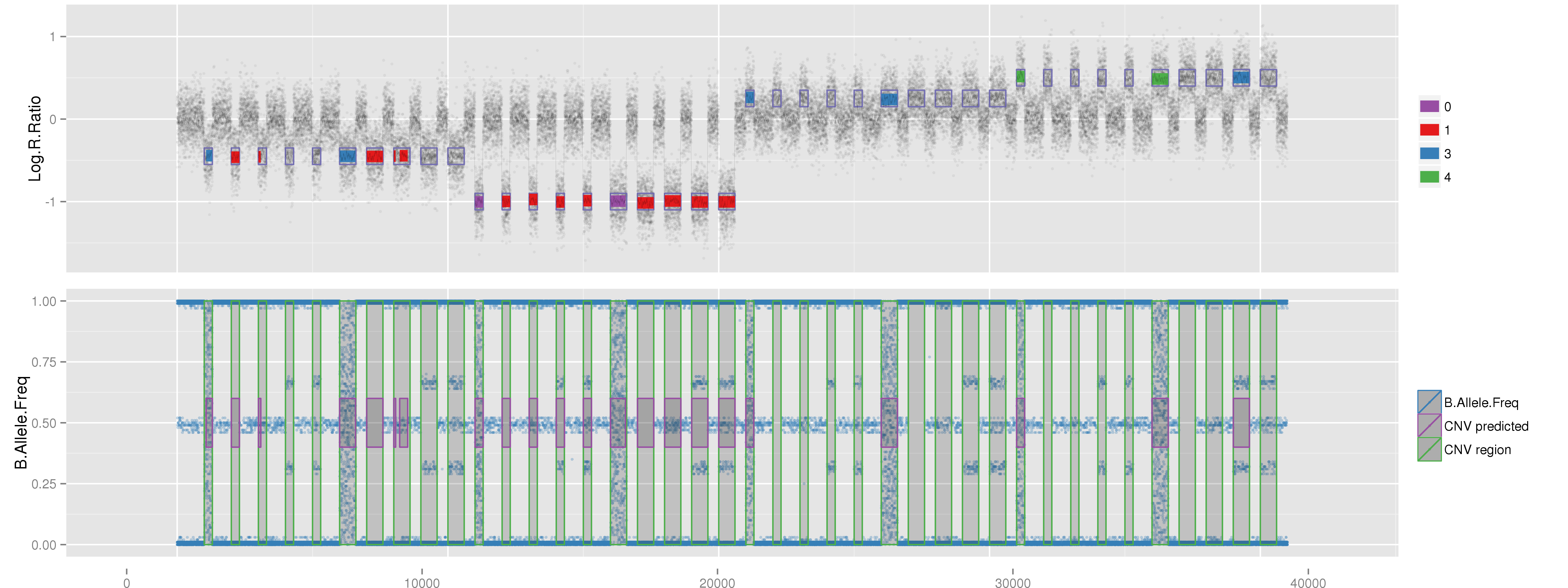
LongRoi <- MakeLongMockSample(Mean=c(-0.6, -0.3, 0.3, 0.6), Size=c(200, 400, 600))
# GADA
Sample <- read.table("LongMockSample.tab", sep="\t", header=TRUE, stringsAsFactors=F)
Gada <- RunGada(Sample)
Gada$ID <- "LongMockSample.tab"
PlotLRRAndCNVs(Gada, tmp=Sample, Name="GadaLong.png", CNVMean=0.3, Roi=LongRoi)
Gada prediction on long mock.
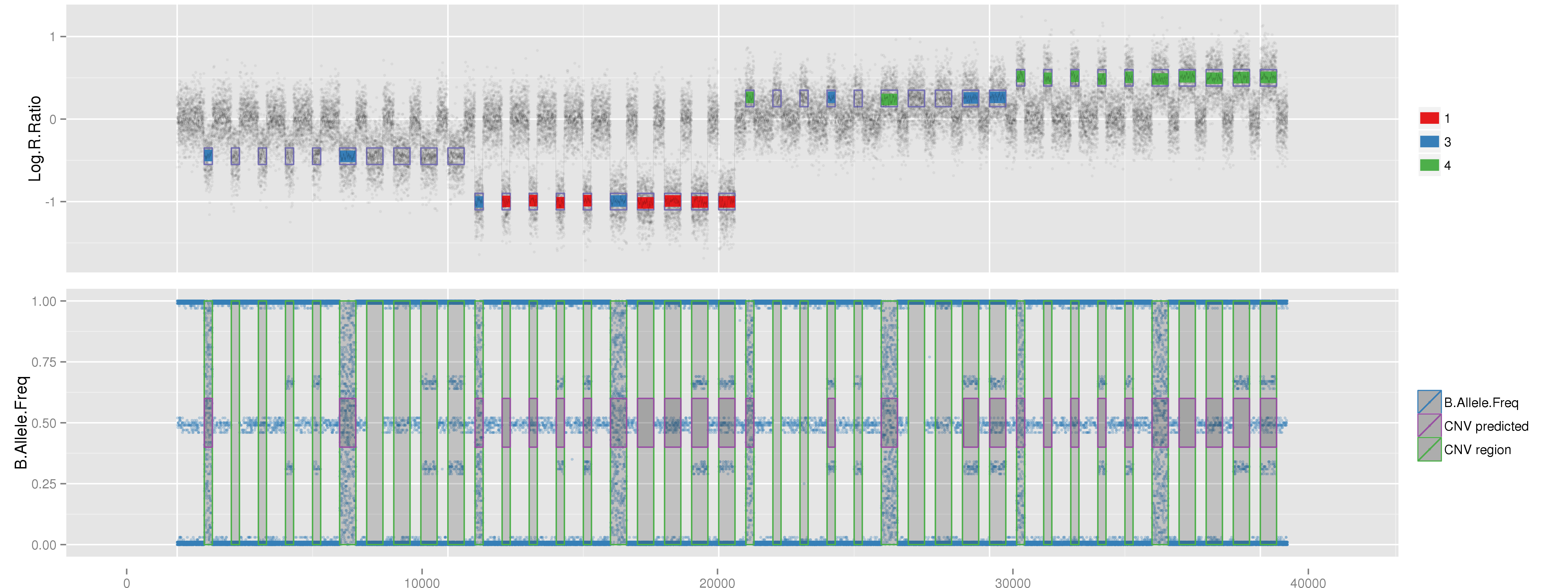
Gada.filter <- FilterFromCNVs(CNVs=Gada, PathRawData=".", MinNumSNPs=10, Source="Gada", Skip=0, Cores=1)
PlotLRRAndCNVs(Gada.filter, tmp=Sample, Name="Gada.filter.Long.png", CNVMean=0.3, Roi=LongRoi)
Gada filtered prediction on long mock.
# PennCNV
LongRoi <- MakeLongMockSample(Mean=c(-0.6, -0.3, 0.3, 0.6), Size=c(200, 400, 600))
Sample <- read.table("LongMockSample.tab", sep="\t", header=TRUE, stringsAsFactors=F)
CNVs <- RunPennCNV(PathRawData=".", Pattern="^LongMockSample.tab$", Skip=0,
Path2PennCNV="/home/programs/penncnv.tardis/penncnv/",
HMM="/home/programs/penncnv.tardis/penncnv/lib/hhall.hmm")
PlotLRRAndCNVs(CNV=CNVs, Sample=Sample, Name="PennCNVLong.png", Roi=LongRoi)
PennCNV prediction on long mock.
PennCNV.filter <- FilterFromCNVs(CNVs=CNVs, PathRawData=".", MinNumSNPs=10, Source="PennCNV", Skip=0, Cores=1)
PlotLRRAndCNVs(CNV=PennCNV.filter, Sample=Sample, Name="PennCNV.Long.filter.png", Roi=LongRoi)
PennCNV filtered prediction on long mock.
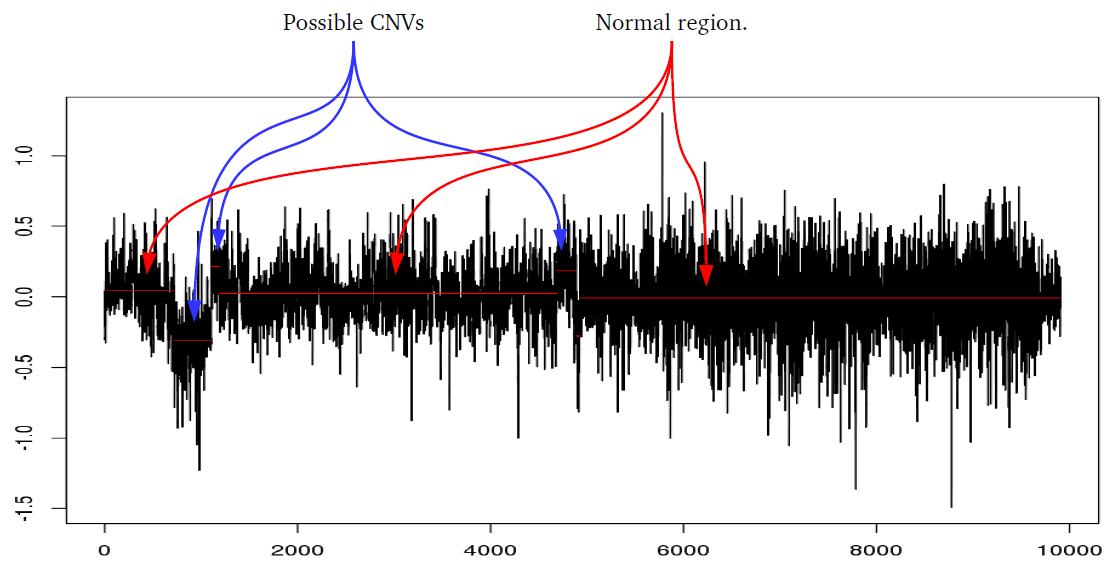
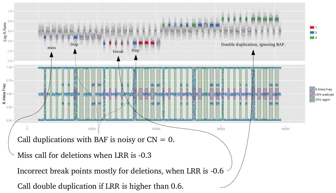
Amplified DNA from dried blood spots offers number of challenges for copy number of variation detection. Here we describe some of the challenges one can find working with DBS data.
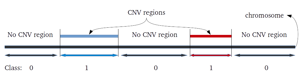
Evaluation of CNV prediction performance is an important step for methods comparison. Here we describe how binary classification is used to evaluate the method performance.
iPsychCNV is an open source R package project. People are welcome to give suggestions, code new functions and/or improve existing ones. The source code is available at Github .
About iPsychCNV
iPsychCNV is a method to find copy number variation from amplified DNA from dried blood spots on Illumina SNP array. It is designed to handle large variation on Log R ratio, and uses B allele frequency to improve CNV calls. iPsychCNV is an open source project on Github
About iPSYCH
The project will study five specific mental disorders; autism, ADHD, schizophrenia, bipolar disorder and depression. All disorders are associated with major human and societal costs all over the world. The iPSYCH project will study these disorders from many different angles, ranging from genes and cells to population studies, from fetus to adult, from cause to symptoms of the disorder, and this knowledge will be combined in new ways across scientific fields, visit iPSYCH.